Electrical component/device that used to amplify signal is called amplifier. The Op-Amp is a type of amplifier that common used in many application. Today we can find the Op-Amp as an IC (integrated circuit).
Picture 1: Symbol of Operational Amplifier
The circuit symbol for an op-amp is shown above, where:
V+ : non-inverting input
V– : inverting input
VOUT : output
VS+ : positive power supply
VS– : negative power supply
If we connect the input to the V+, we can get that the output have the same phase with the input. But if we connect the input to the V–, the output will have phase that opposite of the intput phase.
The power supply pins (and) can be labeled in different ways (See IC power supply pins). Despite different labeling, the function remains the same — to provide additional power for amplification of the signal. Often these pins are left out of the diagram for clarity, and the power configuration is described or assumed from the circuit.
Some modes of Op-Amp circuit:
B. Development History Op-Amp
Op-Amp is a type of differential amplifier. The other type of differential amplifier built from Op-Amp, except the fully differential Op-Amp. The name Operatational Amplifier is used based on the early function that to do some mathematical operational such as summing, difference/subtracting, intregration, or differential.
Op-Amp terdiri atas beberapa jenis, yaitu:
- 1941: First (vacuum tube) op-amp
The first op-amp design for a general-purpose, DC-coupled, high gain, inverting feedback amplifier. This design used three vacuum tubes to achieve a gain of 90 dB and operated on voltage rails of ±350 V. It had a single inverting input rather than differential inverting and non-inverting inputs, as are common in today's op-amps.
It is found in U.S. Patent 2,401,779 "Summing Amplifier" filed by Karl D. Swartzel Jr. of Bell labs in 1941. This design proved its value by being liberally used in the M9 artillery director. The artillery director worked with the SCR584 radar system to achieve extraordinary hit rates (near 90%) that would not have been possible otherwise. [Jung, Walter G. (2004). "Chapter 8: Op Amp History". Op Amp Applications Handbook. Newnes. p. 777]
- 1947: First op-amp with an explicit non-inverting input
In 1947, the name of Operational Amplifier is first formally defined in a paper by Professor John R. Ragazzini, a professor from Columbia University. In the paper a footnote, Ragazzini mentioned that the op-amp design by Loebe Julie (one of his student) would turn out to be quite significant. This op-amp was superior in a variety of ways, but its had two major innovations. The first is input stage used a long-tailed triode pair with loads matched to reduce drift in the output. Second, that more importantly, was the first op-amp design to have two inputs (one inverting, the other non-inverting). This differential input made a whole range of new functionality possible, but it would not be used for a long time due to the rise of the chopper-stabilized amplifier.[ Jung, Walter G. (2004). "Chapter 8: Op Amp History". Op Amp Applications Handbook. Newnes. p. 779]
- 1949: First chopper-stabilized op-amp
In 1949, Edwin A. Goldberg designed a chopper-stabilized op-amp.[ Jung, Walter G. (2004). Op Amp Applications Handbook. Newnes]. The chopper gets an AC signal from DC by switching between the DC voltage and ground at a fast rate (60 Hz or 400 Hz). The advantage of this Op-Amp was improved the gain while significantly reducing the output drift and DC offset. Unfortunately, any design that used a chopper couldn't use their non-inverting input for any other purpose. Techniques that used the non-inverting input regularly would not be popular until the 1960s when op-amp ICs started to show up in the field.
Picture 2: GAP/R’s K2-W Vacume tube op-amp
In 1953, vacuum tube op-amps produced commercially. The op-amp available in the K2-W model and K2-P (chopper add-on available that would effectively eliminate the non-inverting input). The vacume tube op-amp was based on Loebe Julie's (1947) design of op-amp and. This commercially op-amp would start the widespread use of op-amps in industry.
- 1961: First discrete IC op-amps
The birth of transistor in 1947 and silicon transistor in 1954 has made “the dream” of Integrated Circuits (ICs) became a reality. Planar process introduced in 1959 made transistor and ICs stable enough to be commercially useful. Then GAP/R's model P45 (solid-state, discrete op-amps) were being produced in 1961.
Picture 3: GAP/R's model P45 (solid-state, discrete op-amps in 1961)
These op-amps were effectively small circuit boards with packages such as edge-connectors. They usually had hand-selected resistors in order to improve things such as voltage offset and drift. The P45 (1961) had a gain of 94 dB and ran on ±15 V rails. It was intended to deal with signals in the range of ±10 V.
- 1962: First op-amps in potted modules
Picture 4: GAP/R's model PP65 (a solid-state op-amp in a potted module)
The op-amp circuit became more generally use in many industry and many device. Several companies were try to made the op-amp into a single black box so it could be easily threated as a single component. One of the result, in 1962, was GAP/R's model PP65, a solid-state op-amp in a potted module.
- 1963: First monolithic IC op-amp
In 1963, the first monolithic IC op-amp, the μA702 designed by Bob Widlar at Fairchild Semiconductor, was released. Monolithic ICs just a single piece of chip. Its is different from a chip and discrete parts (a discrete IC), or multiple chips bonded and connected on a circuit board (a hybrid IC). Almost all modern op-amps are monolithic ICs; however, this first IC did not meet with much success. Some problem such as an uneven supply voltage, low gain and a small dynamic range held off the dominance of monolithic op-amps. But the problems had been solved in 1965, when the μA709 (also designed by Bob Widlar) was produced.
- 1966: First varactor bridge op-amps
Since the 741, there have been many different directions taken in op-amp design. Varactor bridge op-amps started to be produced in the late 1960s. They were designed to have extremely small input current and are still amongst the best op-amps available in terms of common-mode rejection with the ability to correctly deal with hundreds of volts at their inputs.
- 1968: Release of the μA741
Further improvement in monolithic op-amp result in release of the LM101 in 1967, which solved a variety of issues. This is followed by the μA741 in 1968. The μA741 was extremely similar to the LM101, except that Fairchild's facilities allowed them to include a 30 pF compensation capacitor inside the chip. so it didn’t required external compensation. This simple difference has made the 741 as a legendary op-amp and many modern amplifiers base their pinout on the 741’s. The μA741 is still in production, and has become ubiquitous in electronics — many manufacturers produce a version of this classic chip, recognizable by part numbers containing 741.
- 1970: First high-speed, low-input current FET design
After 741 the derection of improvement were focus high speed and low-input current design. The design started to be made by using FETs, however, it would be largely replaced by op-amps made with MOSFETs in the 1980s. During the 1970s single sided supply op-amps also became available.
- 1972: Single sided supply op-amps being produced
A single sided supply op-amp is one where The input and output voltages of a single sided supply can be as low as the negative power supply. This make the op-amp can operate in many applications with the negative supply pin being connected to the signal ground. It was eliminating the need for a separate negative power supply.
In 1972, the LM324, one such op-amp that came in a quad package (four separate op-amps in one package), was released and became an industry standard As the properties of monolithic op-amps improved, the more complex hybrid ICs were quickly relegated to systems that are required to have extremely long service lives or other specialty systems.
- Recent trends
Recently supply voltages in analog circuits have decreased (near voltages they have in digital logic) and low-voltage op-amps have been introduced reflecting this. Supplies of ±5 V and increasingly 5 V are common. The modern op-amp signal can range from lowest supply voltages to the highest, either input or output.
An ideal op-amp is usually considered to have the following properties, and they are considered to hold for all input voltages:
a. Infinite open-loop gain (when doing theoretical analysis, a limit may be taken as open loop gain AOL goes to infinity);
b. Infinite voltage range available at the output, Vout. In practice the voltages available from the output are limited by the supply voltages VS+ and VS– . The power supply sources are called rails.
c. Infinite bandwidth (i.e., the frequency magnitude response is considered to be flat everywhere with zero phase shift).
d. Infinite input impedance (so, in the diagram, Rin = ∞, and zero current flows from v+ to v–).
e. Zero input current (i.e., there is assumed to be no leakage or bias current into the device).
f. Zero input offset voltage (i.e., when the input terminals are shorted so that v+ = v–, the output is a virtual ground or vout = 0).
g. Infinite slew rate (i.e., the rate of change of the output voltage is unbounded) and power bandwidth (full output voltage and current available at all frequencies).
h. Zero output impedance (i.e., Rout = 0, so that output voltage does not vary with output current).
i. Zero noise.
j. Infinite Common-mode rejection ratio (CMRR).
k. Infinite Power supply rejection ratio for both power supply rails.
All of this ideals can be summarized by the two "golden rules":
I. The output attempts to do whatever is necessary to make the voltage difference

between the inputs zero. à (V+ – V– = 0 or V+ = V– )
This rule only applies in the usual case where the op-amp is used as inverting design (negative feedback). These rules are commonly used as good first approximation for analyzing or designing op-amp circuits.
II. The inputs draw no current. à (i+ = i– = 0).
The real is none of these ideals can be perfectly realized, and various shortcomings and compromises have to be accepted. Depending on the parameters of interest, a real op-amp may be modeled to take account of some of the non-infinite or non-zero parameters using equivalent resistors and capacitors in the op-amp model. The designer can then include the effects of these undesirable, but real, effects into the overall performance of the final circuit. Some parameters may turn out to have negligible effect on the final design while others represent actual limitations of the final performance, that must be evaluated.
D. Basic Design Circuit with Op-Amp for Amplifier
- Inverting Amplifier
It is called inverting amplifier because the design connect the input to the inverting pin of the Op-Amp.
Picture 5: Schematic of inverting amplifier
We can analized the scheme above using the golden rule to get the value of amplification.
I. V* = 0 or V+ = V– , because of V+ connect to the ground so: V+ = V– = 0
II. i+ = i– = 0
From the kirchoff law’s i1 + i2 = i – ,so:
Insert equation 4 and 5 into equation 3 we can get the relation of the input and the output voltage, as a function of the resistances:
- Non-Inverting Amplifier
Picture 6: Schematic of non-inverting amplifier
As same as non-inverting amplifier, we can analized the scheme above using the golden rule to get the value of amplification.
I. V* = 0 or V+=V– , because of V+ connect to the source so: V– = V+ = Vi
II. i+ = i– = 0, so all of the current flowing through R2 also flowing through R1. Therefore, R2 and R1 can be approximated such voltage devider circuit as shown by the scheme below:
Picture 7: Schematic of voltage devider
Now we can use the voltage devider as shown in the equation below:
As we know in the first rule, so the output voltage are:
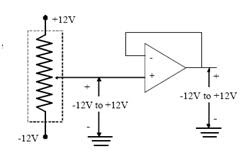
- Voltage / unity follower
Picture 8: Voltage Follower
The voltage follower, also known as a pre-amplifier, is a unity gain amplifier circuit with a short circuit in the feedback path, as shown in Figure 5.16, such that:
It has a very high input impedance and its main application is to reduce the load on the measured system. It also has a very low output impedance that is very useful in some impedance-matching applications.
- Common Mode
Figure 5.12 shows a common amplifier configuration that is used to amplify the small difference that may exist between two voltage signals VA and VB. These may represent, for example, the pressures either side of an obstruction device put in a pipe to measure the volume flow rate of fluid flowing through it. The output voltage 0 is given by:
A differential amplifier is also very useful for removing common mode noise voltages. Suppose VA and VB in Figure 5.12 are signal wires such that VA = +Vs volts and VB = 0 volts. Let us assume that the measurement circuit has been corrupted by a common mode noise voltage Vn such that the voltages on the +Vs and 0V signal wires become (Vs + Vn) and (Vn). The inputs to the amplifier V1 and V2 and the output V0 can then be written as:
So the output will be:
Hence:
If the resistance value are chosen carefully such that R4/R2 = R3/R1, then the equation above simplifies to:
In this example, the voltage noise has been removed (Alan S. Morris. 2001. Measurement and Instrumentation Principles, Third Edition. Butterworth-Heinemann). But in the real case we can’t make the R4/R2 perfectly the same as R3/R1, we just make both fraction value near each other. The output of a real differential amplifier is better described as:
where Acm is the common-mode gain or the gain of noice, which is typically much smaller than the differential gain Ad.
The CMRR is defined as the ratio of the powers of the differential gain over the common-mode gain, measured in positive decibels (thus using the 20 log rule):
The CMRR is a very important specification, as it indicates how much of the common-mode signal will appear in your measurement. The value of the CMRR often depends on signal frequency as well, and must be specified as a function there of.
It is often important in reducing noise on transmission lines. For example, when measuring the resistance of a thermocouple in a noisy environment, the noise from the environment appears as an offset on both input leads, making it a common-mode voltage signal. The CMRR of the measurement instrument determines the attenuation applied to the offset or noise (
http://en.wikipedia.org/wiki/Common-mode_rejection_ratio, 11
th April 2011. 10:38 PM).
E.Operational and Other Design Circuit with Op-Amp
- Summing amplifier
Picture 9: Summing amplifier
From the golden rule:
I. V* = 0 or V+=V– , because of V+ connect to the ground so: V– = V+ = 0
II. i+ = i– = 0, so
And from kirchoff’s law, we know that the current enter point A is the same as the current leave that point.
Insert the voltage devider, the equation above can be write as:

Based on the golden rule, we can approximate the equation as:
Special case:
· If we assume or make the R1=R2=Rn=R, where Rn and Vn connect to the point A the fuction of output voltage is:
- Subtractor / Diferential amplifier
This is the combining of inverting and non-inverting design of operational amplifiers. All the input connect to the inverting pin will subtract all the input that connect to the non-inverting pin. This in because the inverting pin will produce the inverted output signal from all sources connect to the pin.
Picture 10: Scheme of subtractor/diferential amplifier
From the golden rule:
I. V* = 0 or V+=V–
II. i+ = i– = 0, so
We can get two more equation. First is the equation for inverting side:
The second equation is for the non-inverting side, that can be approximate as the voltage devider.
Using the first rule of golden rule we can combine this two equation (equ.19 and equ. 20) as:
For a special case where the Rg/R2=Rf/R1=K, the equation can be simplify:
- Differentiator
The basic of analizing this circuit is using the golden rule.
I. V* = 0 or V+ = V– , because of V+ connect to the ground so: V+ = V– = 0
II. i+ = i– = 0
Picture 11: Differentiator Amplifier
From the kirchoff's law, we can get:

- Integrator
Picture 12: Integrator Amplifier
The basic of analizing this circuit is using the golden rule.
III. V*= 0 or V+=V– , because of V+ connect to the ground so: V+=V–= 0
IV. i+ = i– = 0
From the kirchof, we can get:
Using the golden rule:
- Penguat untuk instrumentasi (Instrumentation amplifier)
An instrumentation amplifier is a differential op-amp circuit providing high input impedances with ease of gain adjustment through the variation of a single resistor
Picture 13: Instrumentation Amplifier
This intimidating circuit is constructed from a buffered differential amplifier stage with three new resistors linking the two buffer circuits together. Consider all resistors to be of equal value except for RG or Rgain. The negative feedback of the upper-left op-amp causes the voltage at point 1 (top of Rgain) to be equal to V1. Likewise, the voltage at point 2 (bottom of Rgain) is held to a value equal to V2. This established a voltage drop across Rgain equal to the voltage difference between V1 and V2. That voltage drop causes a current through Rgain, and since the feedback loops of the two input op-amps draw no current, that same amount of current through Rgain must be going through the two "R" resistors above and below it. This produces a voltage drop between points 3 and 4 equal to:

The regular differential amplifier on the right-hand side of the circuit then takes this voltage drop between points 3 and 4, and amplifies it by a gain of 1 (assuming again that all "R" resistors are of equal value). Though this looks like a cumbersome way to build a differential amplifier, it has the distinct advantages of possessing extremely high input impedances on the V1 and V2 inputs (because they connect straight into the noninverting inputs of their respective op-amps), and adjustable gain that can be set by a single resistor. Manipulating the above formula a bit, we have a general expression for overall voltage gain in the instrumentation amplifier:

Though it may not be obvious by looking at the schematic, we can change the differential gain of the instrumentation amplifier simply by changing the value of one resistor: Rgain. We could still change the overall gain by changing the values of some of the other resistors, but this would necessitate balanced resistor value changes for the circuit to remain symmetrical. Please note that the lowest gain possible with the above circuit is obtained with Rgain completely open (infinite resistance), and that gain value is 1.
*Thanks*